Abstraction Barriers : Boundaries Giving Base To Data Abstraction

You can read about data abstraction in my previous post ,in this blog I’ll talk about the abstraction barriers.When we represent a rational numbers in terms of pair with operations like make-rat and selectors like numer and denom .Basic idea behind data abstraction is to identify for each type of data object a basic set of operations in terms of which all manipulations of data object can be expressed and then using those procedures to manipulate the data.

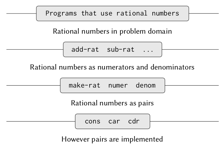
In above figure as you can see that we have levels of abstraction which fulfills different needs. But these levels are divided by horizontal boundaries which are known as Abstraction barriers. Different levels are isolated from each other. At each level , the barrier seperates the programs(above) that use the data abstraction from the program below, that implement data abstraction. As we can see from figure that we started from root level i.e primitive level and regularly abstracting different levels which doesn’t care about how below level is implemented. Programs at the top level only uses public procedure like add-rat , sub-rat ,mul-rat etc. These procedures are implemented in terms of make-rat ,numer,denom etc which are again implemented in terms of pairs.We can say that procedures at each level are interfaces that define abstraction barriers and connect the different levels.

So creating abstraction barriers is a simple idea, but the biggest advantage of it – makes program much easier to maintain and modify.But one disadvantage is the representation of data/procedures influences the program that operate on it, therefore slight change in representation can modify corresponding procedure accordingly. So this change could be expensive and time consuming if there is large program and this will depend on what level change is happening like if the change is at ground level it will be more expensive and time consuming compare to change at higher level. So we have to confine design to fewer program modules and try to make it less dependent on representation.

So abstraction barrier is one of the steps to do data abstraction in your program.

Procedural Abstraction

Definition of ‘Abstraction’ : the quality of dealing with ideas rather than events.

You can read about Abstraction and data abstraction in my previous blog post.

In this blog post we’ll learn about Procedural Abstraction, Procedural Abstraction is something like dividing the complex problem into subproblems and implementing it through sub procedures.

Procedural abstraction is not simply that one is dividing the program into parts.After all , we could take any large program and divide the program into parts – the first ten lines,next ten lines and so on.It is crucial that each procedure accomplishes an identifiable task(i.e represents an idea) that can be used as a module in defining other procedure.For example we are defining a procedure named good-enough?  ,

(define (good-enough? guess x)
  (< (abs (- (square guess) x)) 0.001))

In above example we are using sqaure as black box i.e it is doing something but we are not concerned with how it is doing. The details of how square is computed can be suppressed, to be considered at a later time.Indeed, as far as the good-enough? procedure is concerned, square is not quite a procedure but rather an abstraction of a procedure, a so-called procedural abstraction. So the person which is implementing good-enough? doesn’t care about how square is working he can fully concentrate upon good-enough? which will create abstraction.

One of the biggest advantages of procedural abstraction is many users can work upon different modules due to which efficiency of team could be increased.We can hide details and gives us the building block that can be reused in other situation.We can easily replace implemetation by better ones.

To summarise, procedural abstraction is a way to implement abstraction and each sub-procedure should represent an idea.

Finding Roots By Half Interval Method

The half interval method is the most basic method to find roots of an equation i.e to find x such  that f(x) = 0 , where f is a continuos function. Now the idea is if we have two points a and b such that f(a) < 0 < f(b) then f must have  atleast one zero between  a and b. So to locate a zero we’ll take average of  a and b and compute f(x) where x is average of a and b.If f(x) > 0,then f must have zero between a and x.If f(x) < 0 , then f must have zero between x and b.So we continue this way to identify smaller and smaller intervals on which f must have  a zero.Therefore when we reach a point where interval is small enough the process stops. Since we are calculating average at each level and decreasing our level of uncertainity by half , the number of steps required grows as O (log (L/T)) ,where L is the length of original interval i.e difference of a and b and T is the error tolereance (size of interval we consider small enough).

(define (search f neg-point pos-point)
  (let ((midpoint (average neg-point pos-point)))
    (if (close-enough? neg-point pos-point)
        midpoint
        (let ((test-value (f midpoint)))
          (cond ((positive? test-value)
                  (search f neg-point midpoint))
                ((negative? test-value)
                 (search f midpoint pos-point))
                (else midpoint))))))

Above pseudo-code is taken from Structure And Interpretation of Computer Programs.Now the close-enough? used above which is breaking condition for the recursive function will be :

(define (close-enough? x y)
  (< (abs (- x y)) 0.001))

close-enough? function will decide how much accurate will be our answer.

To summarise we are getting roots of the equation in O(log (L/T)) by half-interval method.

Tail Call Optimisation: A way to avoid Overflow of Stack

Tail Call optimisation
Tail call optimisation is compiler based optimisation ,it is used to avoid allocating new stack space in case of recursive call in function.So let’s see what happens in tail call optimisation. When a function is called, the computer must “remember” the place it was called from, the return address, but in case of tail call the new called function is not alloted with a new stack space instead it replaces the the calling function in the same stack due to which stack overflow can be avoided.Most of the funtional program support tail call optimisation.For function having tail call optimisation it should have the proper implementation. Let’s see by example how to write tail call optimisation:

(define (fact x)
  (if (= x 0) 1
      (* x (fact (- x 1)))))

Above implementation of factorial doesn’t do tail call optimisation because when the recursive call is made, the function needs to keep track of the multiplication it needs to do with the result after the call returns.

(fact 3)
(* 3 (fact 2))
(* 3 (* 2 (fact 1)))
(* 3 (* 2 (* 1 (fact 0))))
(* 3 (* 2 (* 1 1)))
(* 3 (* 2 1))
(* 3 2)
6